STAC, xarray and dask
This tutorial demonstrates how to load satellite images from a SpatioTemporal Asset Catalog (STAC), create an xarray cube from them, and run a computation using dask. For those who don't intend to use xarray and dask, the tutorial generally demonstrates how to find earth observation data on our systems using the STAC metadata catalog and Python.
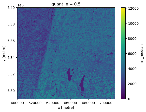
As an example, the temporal median of Sentinel-2 L2A data acquired over Munich in 2022 is computed, stored in a Zarr file, and visualized.
Setting up the JupyterLab environment
This demo is intended to run in a Jupyter notebook with a JupyterLab instance inside a SLURM job. We are going to use the terrabyte Portal to set this up.
First we will create a mamba environment and install all Python packages required to run the notebook. For this, we will start JupyterLab based on micromamba and the pre-configured environment terrabyte_base.
Click on Jupyter Notebook in the portal (e.g. under Apps) and configure the following (the micromamba version may change):
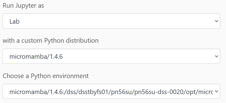
(full path to the environment:
micromamba/<version>:/dss/dsstbyfs01/pn56su/pn56su-dss80020/micromamba/envs/terrabyte_base)
You may leave the rest unchanged and then launch the notebook. It will take a little moment and you can then start the session.
Once connected, start a Jupyter notebook from the Launcher menu. Here we execute the code to create our mamba environment "myenv" (or any name you prefer) with all Python packages needed for the tutorial:
!micromamba create -y -n myenv jupyter xarray rioxarray odc-stac odc-geo pystac-client dask folium geopandas zarr jupyter-server-proxy
Once installation has finished (it will take a while), you may close this JupyterLab session and return to the terrabyte portal.
Here, you can now select the newly created micromamba environment to start our actual JupyterLab session:
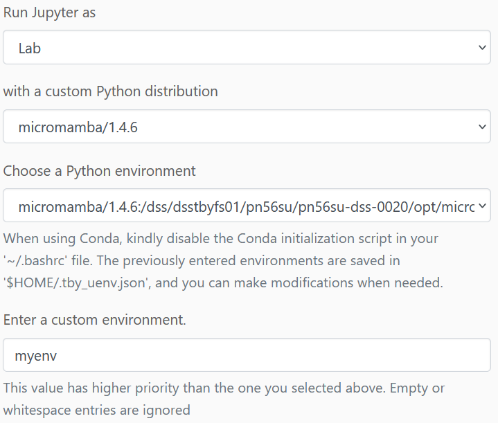
Here it is also worth defining a larger amount of resources for accelerating the computation.
Once the JupyterLab is started you can begin with the tutorial.
A short word on STAC
STAC is the central way of accessing any spatio-temporal data on terrabyte. See here for an introduction and the detailed sepcification:
In principal, data is offered as a catalog containing data from various sources. This catalog is further sub-divided into collections. A collection could for example contain a certain satellite data product like Sentinel-1 GRD, SLC or Sentinel-2 L2A. Each collection consists of multiple items, which might represent individual satellite scenes or product tiles (e.g. the MGRS tiles of Sentinel-2). Each item consists of one or many assets, which contain links to the actual data. For example individual GeoTIFF files for each band.
The terrabyte STAC catalog URL is https://stac.terrabyte.lrz.de/public/api.
Further down you will find examples on how to list all available collections and how to query the STAC catalog in Python using the pystac library. The content can also be explored by opening the above link in a browser.
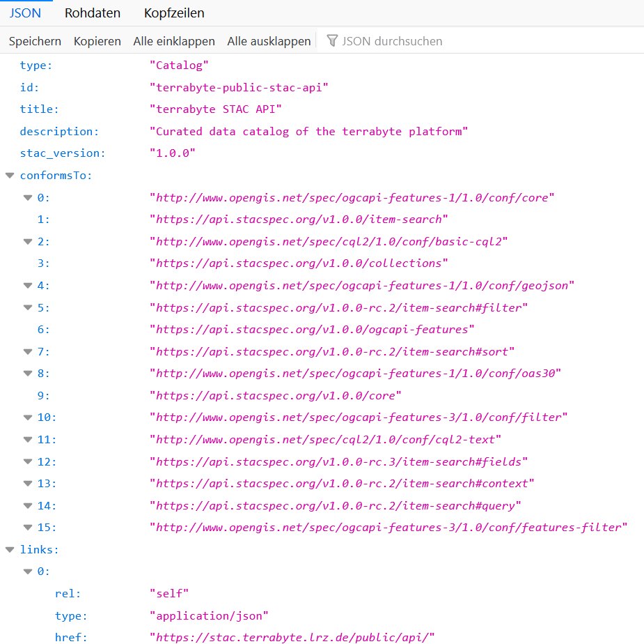
From there you can navigate to individual collections and explore their
metadata content for search queries. For example, under
https://stac.terrabyte.lrz.de/public/api/collections/sentinel-2-c1-l2a/items
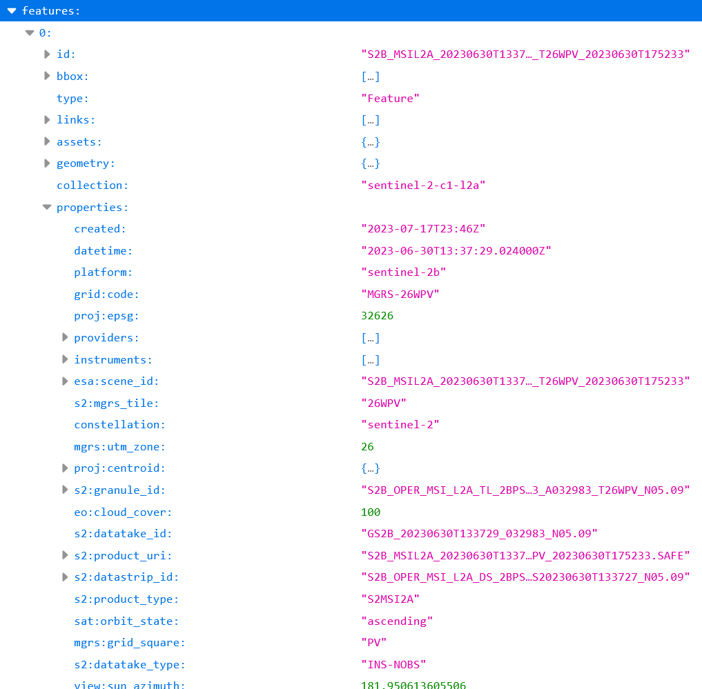
→ features → 0 → properties we can list the properties of the
first item of the sentinel-2-c0-l2a collection. This list contains,
amongst others, the entries eo:cloud_cover and s2:mgrs_tile, which
will be queried in the tutorial below. The namespaces eo, grid, proj,
mgrs, sat and view refer to dedicated
STAC extensions. s2
is a custom namespace for expressing Sentinel-2 specific metadata that
cannot be described in other STAC extensions.
Let's load some Python packages
import os
import socket
import xarray
import rioxarray
from odc import stac as odc_stac
from odc.geo import geobox
from pystac_client import Client as pystacclient
import dask
from dask.distributed import Client
import folium
import folium.plugins as folium_plugins
import geopandas as gpd
Configuration
# the output directory to store the results
# the path may vary depending on your granted DSS storage location
# for now we use the Home Folder ~
dir_out = '~/xarray-dask-tutorial'

# STAC settings
catalog_url = 'https://stac.terrabyte.lrz.de/public/api'
collection_s2 = 'sentinel-2-c1-l2a'

# input data settings
year = 2022
resolution = 60
mgrs = '32UPU'
max_cloud_cover = 60
bands = ['nir', 'red']

# Output data
filename_base = f'S2_y{year}_res{resolution}_{band}_median_{mgrs}.zarr'
filename = os.path.join(dir_out, filename_base)

# dask
dask_tmpdir = os.path.join(dir_out, 'scratch', 'localCluster')
#we use the values supplied when starting the Jupyterlab session
Explore the STAC catalog
catalog = pystacclient.open(catalog_url, ignore_conformance=True)

# list the IDs of all STAC catalog collections
for collection in catalog.get_all_collections():
    print( collection.id)
Query data from the STAC catalog
gte and lte describe greater than or equal and lower than or equal, respectively.
# STAC metadata entries for discovering assets
query = {
    'eo:cloud_cover': {
        "gte": 0,
        "lte": max_cloud_cover
    },
    's2:mgrs_tile': {'eq': mgrs}
}

start = f'{year}-01-01T00:00:00Z'
end = f'{year}-12-31T23:59:59Z'

resultsS2Stac = catalog.search(
    collections=[collection_s2],
    datetime=[start, end],
    query=query
    )

items = list(resultsS2Stac.items())
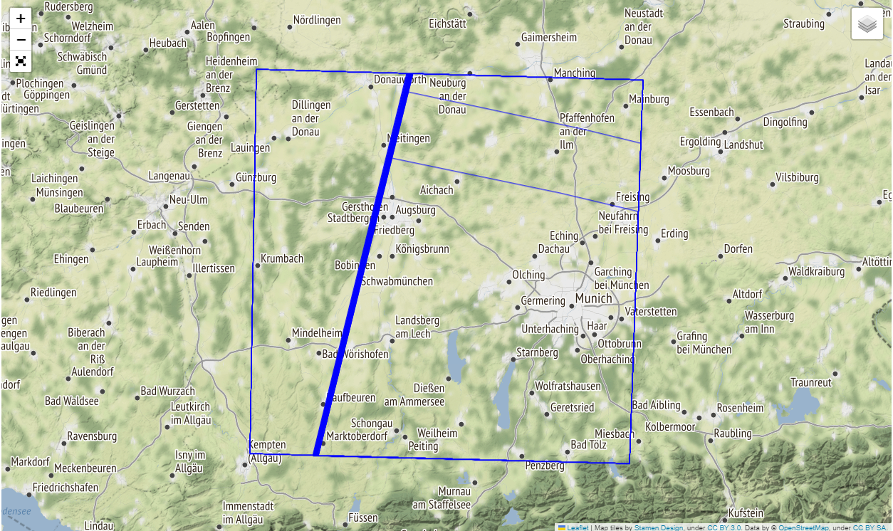
Visualize the covered area
map = folium.Map(tiles='Stamen Terrain')
layer_control = folium.LayerControl(position='topright', collapsed=True)
fullscreen = folium_plugins.Fullscreen()
style = {'fillColor': '#00000000', "color": "#0000ff", "weight": 1}

footprints = folium.GeoJson(
    gpd.GeoDataFrame.from_features([item.to_dict() for item in items]).to_json(),
    name='Stac Item footprints',
    style_function=lambda x: style,
    control=True
)

footprints.add_to(map)
layer_control.add_to(map)
fullscreen.add_to(map)
map.fit_bounds(map.get_bounds())
map
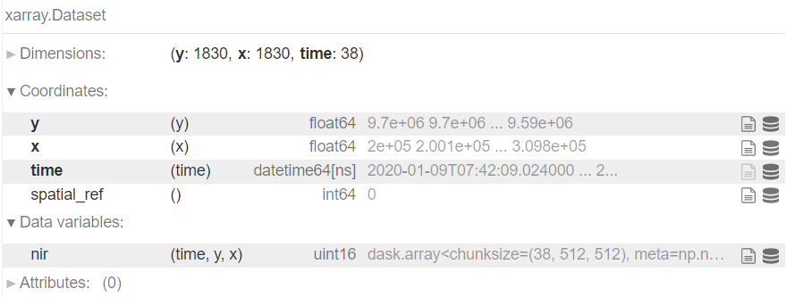
Load the STAC items into xarray
cube = odc_stac.load(
    items,
    bands=[band],
    resolution=resolution,
    stac_cfg=cfg,
    groupby='solar_day',
    chunks={'x': 1024, 'y': 1024}, # spatial chunking
    anchor=geobox.AnchorEnum.FLOATING # preserve original pixel grid
)

# temporal chunking
cube = cube.chunk(chunks={'time': -1})

# write CF-compliant CRS representation
cube = cube.rio.write_crs(cube.coords['spatial_ref'].values)
cube
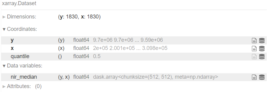
Define the computation
median = cube.quantile(0.5, dim='time', skipna=True, keep_attrs=True)
median = median.rename({b: f'{b}_median' for b in list(cube.keys())})
median
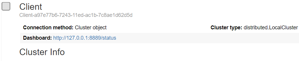
Start the dask client with port forwarding via the jupyter-server-proxy
The client object displayed in the notebook (see example screenshot below) contains a link to the dask dashboard, which can be displayed locally to monitor the progress of the computation once it started.
#get host and port information for the currently running Jupyterlab from Environment Variables
host=os.getenv("host")
JLPort=os.getenv("port")

#create to URL to point to the jupyter-server-proxy
daskUrl=f"https://portal.terrabyte.lrz.de/node/{host}/{JLPort}/proxy/"+"{port}/status"

#dask will insert the port it is running in the {port} part of the URL
dask.config.set({"distributed.dashboard.link": daskUrl})

#set the temporary dir (for intermediate files)
dask.config.set(temporary_directory=dask_tmpdir)

#Dask gets the information on how much CPU/MEM you have selected and sets its workers accordingly
client = Client(threads_per_worker=1)

client
Start the computation
%%time
delayed = median.to_zarr(filename, mode='w', compute=False, consolidated=True)
dask.compute(delayed)
Close the dask cluster
client.cluster.close()
time.sleep(5)
client.close()
Load and visualize the result
result = xarray.open_zarr(filename)
result.to_array().squeeze().plot.imshow()